- Lecturer: Sergio Uribe, Assoc Prof, PhD
- Riga Stradins University, July 2020
Required packages
pacman::p_load(
  car,
  broom,
  tidyverse,
  ggfortify,
  mosaic,
  huxtable,
  jtools,
  latex2exp,
  pubh,
  sjlabelled,
  sjPlot,
  sjmisc
)

theme_set(sjPlot::theme_sjplot2(base_size = 10))
theme_update(legend.position = "top")
# options('huxtable.knit_print_df' = FALSE)
options('huxtable.knit_print_df_theme' = theme_article)
options('huxtable.autoformat_number_format' = list(numeric = "%5.2f"))
knitr::opts_chunk$set(collapse = TRUE, comment = NA)
Epidemiological Descriptive Analysis
Onchocerciasis in Sierra Leone.
data(Oncho)
Oncho %>% head()| id | mf | area | agegrp | sex | mfload | lesions |
|---|---|---|---|---|---|---|
| 1 | Infected | Savannah | 20-39 | Female | 1 | No |
| 2 | Infected | Rainforest | 40+ | Male | 3 | No |
| 3 | Infected | Savannah | 40+ | Female | 1 | No |
| 4 | Not-infected | Rainforest | 20-39 | Female | 0 | No |
| 5 | Not-infected | Savannah | 40+ | Female | 0 | No |
| 6 | Not-infected | Rainforest | 20-39 | Female | 0 | No |
Oncho %>%
  mutate(mf = relevel(mf, ref = "Infected")) %>%
  copy_labels(Oncho) %>%
cross_tab(mf ~ area) | Infection | levels | Infected | Not-infected | Total |
|---|---|---|---|---|
| Total N (%) | 822 (63.1) | 480 (36.9) | 1302 | |
| Residence | Savannah | 281 (34.2) | 267 (55.6) | 548 (42.1) |
| Rainforest | 541 (65.8) | 213 (44.4) | 754 (57.9) |
Table with all descriptive statistics except id and mfload:
Oncho %>%
  # dplyr:select(-c(id, mfload)) %>%
  dplyr::select(-id) %>%
  dplyr::select(-mfload) %>%  # just for example
  mutate(mf = relevel(mf, ref = "Infected")) %>%
  copy_labels(Oncho) %>%
cross_tab(mf ~ area + .) | Infection | levels | Infected | Not-infected | Total |
|---|---|---|---|---|
| Total N (%) | 822 (63.1) | 480 (36.9) | 1302 | |
| Residence | Savannah | 281 (34.2) | 267 (55.6) | 548 (42.1) |
| Rainforest | 541 (65.8) | 213 (44.4) | 754 (57.9) | |
| Age group (years) | 5-9 | 46 (5.6) | 156 (32.5) | 202 (15.5) |
| 10-19 | 99 (12.0) | 119 (24.8) | 218 (16.7) | |
| 20-39 | 299 (36.4) | 125 (26.0) | 424 (32.6) | |
| 40+ | 378 (46.0) | 80 (16.7) | 458 (35.2) | |
| Sex | Male | 426 (51.8) | 190 (39.6) | 616 (47.3) |
| Female | 396 (48.2) | 290 (60.4) | 686 (52.7) | |
| Number of lesions | No | 640 (77.9) | 461 (96.0) | 1101 (84.6) |
| Yes | 182 (22.1) | 19 (4.0) | 201 (15.4) |
Data set about blood counts of T cells from patients in remission from Hodgkin’s disease or in remission from disseminated malignancies. We generate the new variable Ratio and add labels to the variables.
data(Hodgkin)
Hodgkin <- Hodgkin %>%
  mutate(Ratio = CD4/CD8) %>%
  var_labels(
    Ratio = "CD4+ / CD8+ T-cells ratio"
    )

Hodgkin %>% head()| CD4 | CD8 | Group | Ratio |
|---|---|---|---|
| 396 | 836 | Hodgkin | 0.47 |
| 568 | 978 | Hodgkin | 0.58 |
| 1212 | 1678 | Hodgkin | 0.72 |
| 171 | 212 | Hodgkin | 0.81 |
| 554 | 670 | Hodgkin | 0.83 |
| 1104 | 1335 | Hodgkin | 0.83 |
Descriptive statistics for CD4+ T cells:
Hodgkin %>%
estat(~ CD4)| N | Min. | Max. | Mean | Median | SD | CV | |
|---|---|---|---|---|---|---|---|
| CD4+ T-cells | 40.00 | 116.00 | 2415.00 | 672.62 | 528.50 | 470.49 | 0.70 |
- outcome ~ exposure
- ~ outcome | exposure
where, outcome is continuous and exposure is a categorical (factor) variable.
Hodgkin %>%
estat(~ Ratio|Group)| Disease | N | Min. | Max. | Mean | Median | SD | CV | |
|---|---|---|---|---|---|---|---|---|
| CD4+ / CD8+ T-cells ratio | Non-Hodgkin | 20.00 | 1.10 | 3.49 | 2.12 | 2.15 | 0.73 | 0.34 |
| Hodgkin | 20.00 | 0.47 | 3.82 | 1.50 | 1.19 | 0.91 | 0.61 |
descriptive statistics for all variables in the data set:
Hodgkin %>%
  mutate(Group = relevel(Group, ref = "Hodgkin")) %>%
  copy_labels(Hodgkin) %>%
cross_tab(Group ~ CD4 + .)| Disease | levels | Hodgkin | Non-Hodgkin | Total |
|---|---|---|---|---|
| Total N (%) | 20 (50.0) | 20 (50.0) | 40 | |
| CD4+ T-cells | Mean (SD) | 823.2 (566.4) | 522.0 (293.0) | 672.6 (470.5) |
| CD8+ T-cells | Mean (SD) | 613.9 (397.9) | 260.0 (154.7) | 436.9 (347.7) |
| CD4+ / CD8+ T-cells ratio | Mean (SD) | 1.5 (0.9) | 2.1 (0.7) | 1.8 (0.9) |
  # theme_article() %>%
  # add_footnote("Values are medians with interquartile range.")
Inferential statistics
var.test(Ratio ~ Group, data = Hodgkin)

    F test to compare two variances

data:  Ratio by Group
F = 0.6294, num df = 19, denom df = 19, p-value = 0.3214
alternative hypothesis: true ratio of variances is not equal to 1
95 percent confidence interval:
 0.2491238 1.5901459
sample estimates:
ratio of variances
         0.6293991
QQ-plots against the standard Normal distribution.
Hodgkin %>%
qq_plot(~ Ratio|Group) %>%
axis_labs()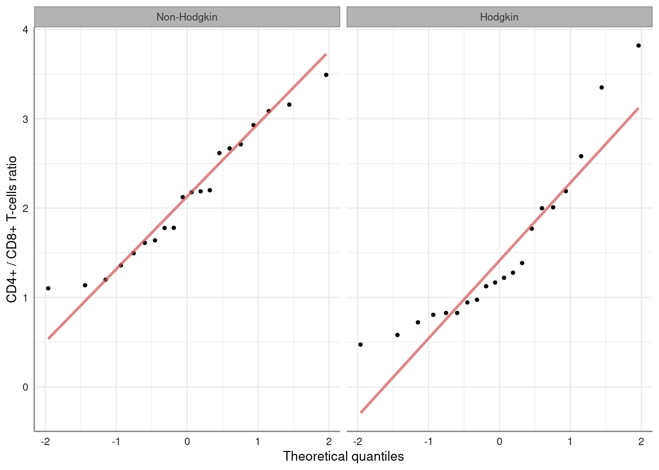 non-parametric test to compare the groups:
wilcox.test(Ratio ~ Group, data = Hodgkin)

    Wilcoxon rank sum test

data:  Ratio by Group
W = 298, p-value = 0.007331
alternative hypothesis: true location shift is not equal to 0
For relatively small samples (for example, less than 30 observations per group) is a standard practice to show the actual data in dot plots with error bars. The pubh package offers two options to show graphically differences in continuous outcomes among groups:
For small samples: strip_error For medium to large samples: bar_error
Hodgkin %>%
  strip_error(Ratio ~ Group) %>%
  axis_labs()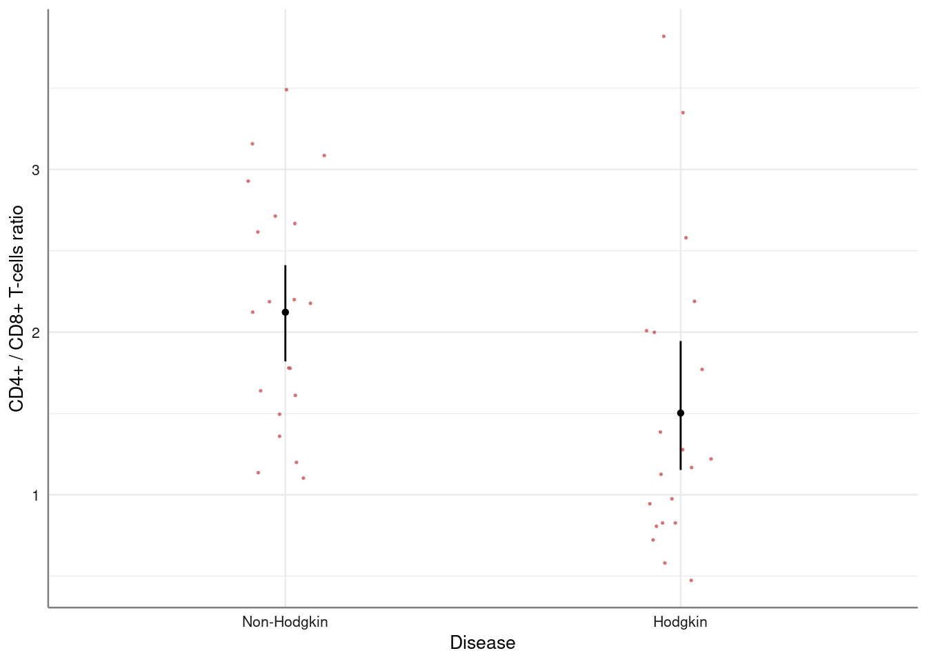
In the previous code, axis_labs applies labels from labelled data to the axis.
The error bars represent 95% confidence intervals around mean values.
Is relatively easy to add a line on top, to show that the two groups are significantly different. The function gf_star needs the reference point on how to draw an horizontal line to display statistical difference or to annotate a plot; in summary, gf_star:
Hodgkin %>%
  strip_error(Ratio ~ Group) %>%
  axis_labs() %>%
  gf_star(x1 = 1, y1 = 4, x2 = 2, y2 = 4.05, y3 = 4.1, "**")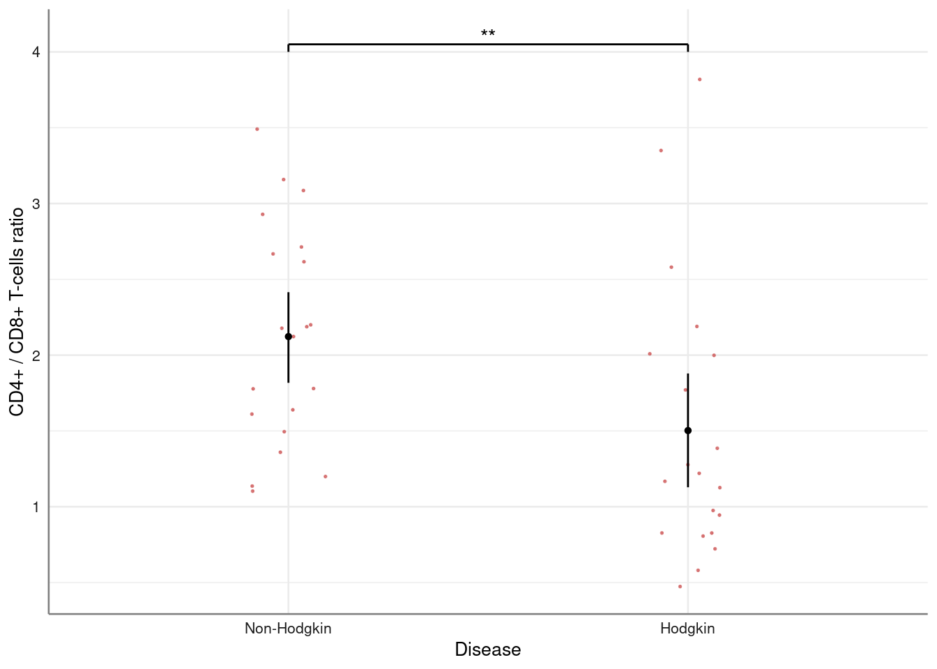
For larger samples we could use bar charts with error bars. For example:
data(birthwt, package = "MASS")
birthwt <- birthwt %>%
  mutate(
    smoke = factor(smoke, labels = c("Non-smoker", "Smoker")),
    Race = factor(race > 1, labels = c("White", "Non-white")),
    race = factor(race, labels = c("White", "Afican American", "Other"))
    ) %>%
  var_labels(
    bwt = 'Birth weight (g)',
    smoke = 'Smoking status',
    race = 'Race',
  )
birthwt %>%
bar_error(bwt ~ smoke) %>%
axis_labs()
No summary function supplied, defaulting to `mean_se()`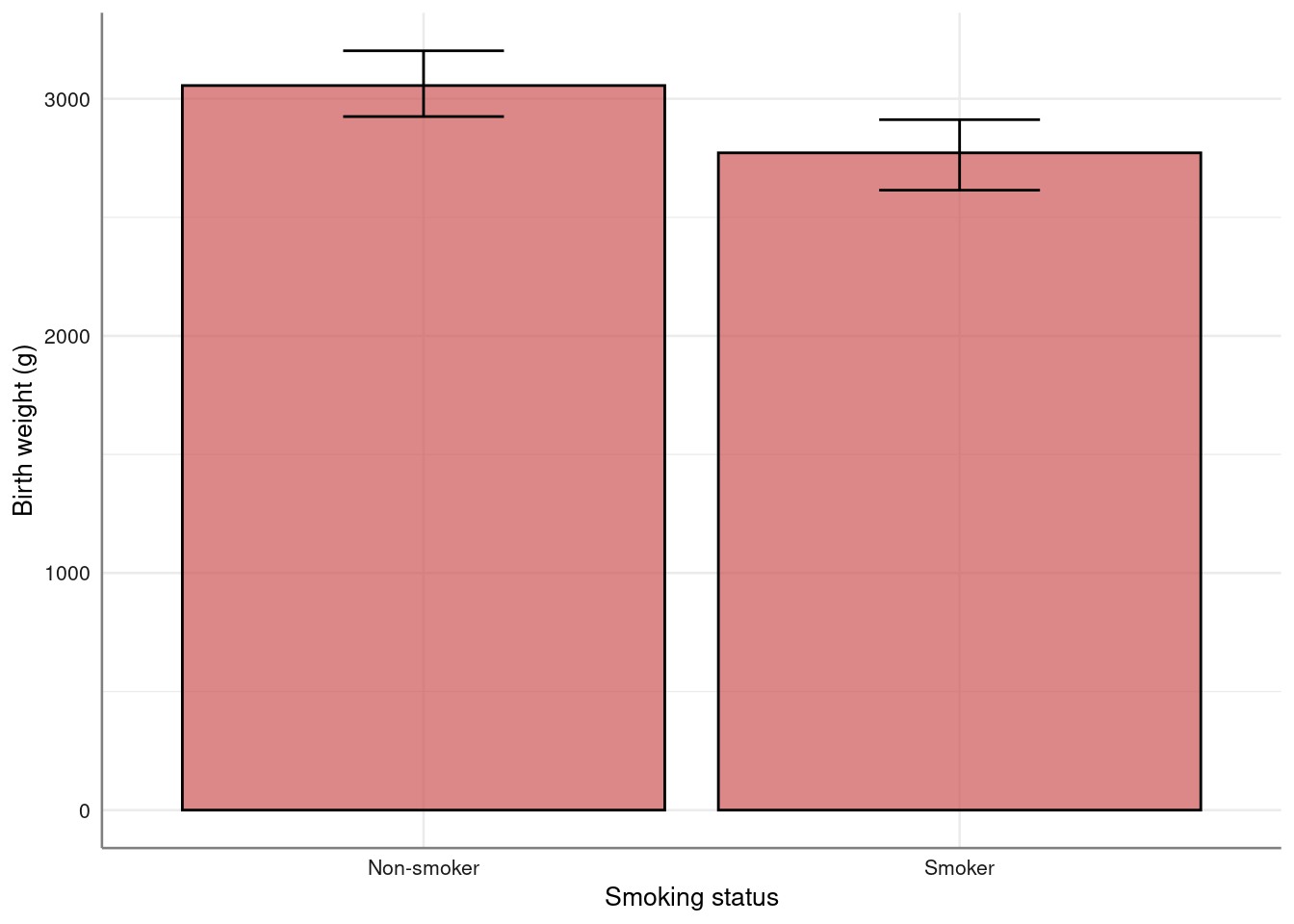
Quick normality check:
birthwt %>%
qq_plot(~ bwt|smoke) %>%
axis_labs()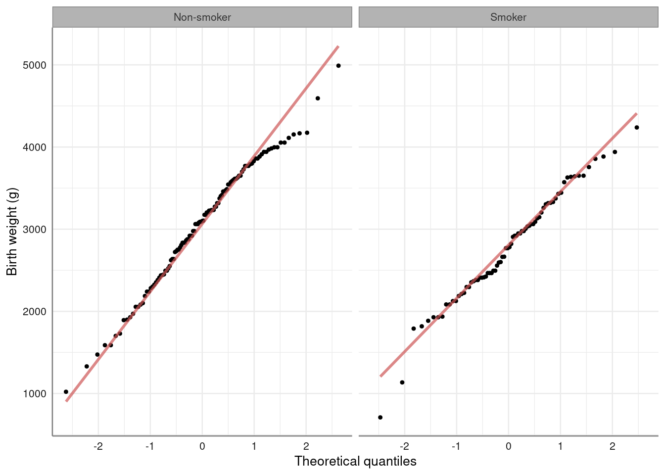 The (unadjusted) t-test:
t.test(bwt ~ smoke, data = birthwt)

    Welch Two Sample t-test

data:  bwt by smoke
t = 2.7299, df = 170.1, p-value = 0.007003
alternative hypothesis: true difference in means is not equal to 0
95 percent confidence interval:
  78.57486 488.97860
sample estimates:
mean in group Non-smoker     mean in group Smoker
                3055.696                 2771.919
Final plot with annotation to highlight statistical difference (unadjusted):
birthwt %>%
bar_error(bwt ~ smoke) %>%
axis_labs() %>%
gf_star(x1 = 1, x2 = 2, y1 = 3400, y2 = 3500, y3 = 3550, "**")
No summary function supplied, defaulting to `mean_se()`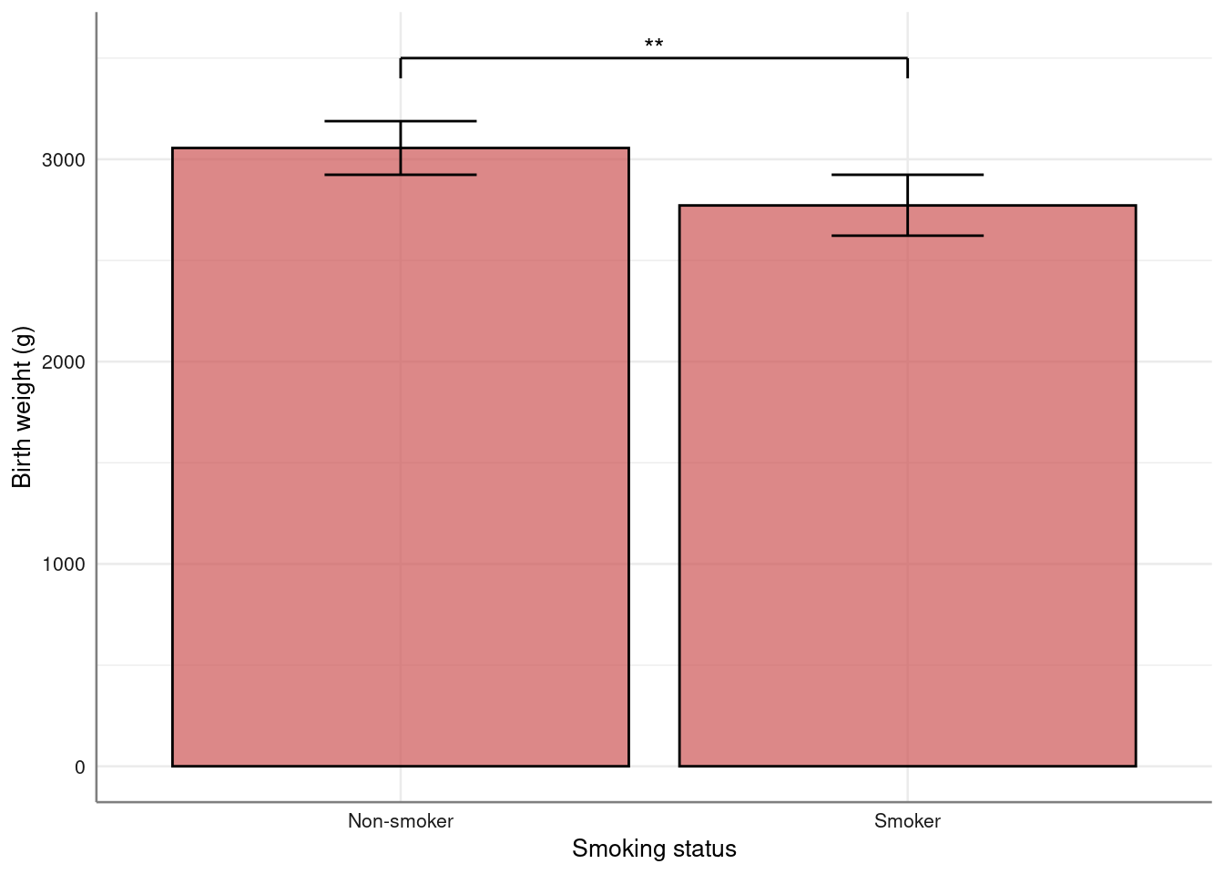 strip_error and bar_error can generate plots stratified by a third variable, for example:
birthwt %>%
  bar_error(bwt ~ smoke, fill = ~ Race) %>%
  gf_refine(ggsci::scale_fill_jama()) %>%
  axis_labs()
No summary function supplied, defaulting to `mean_se()`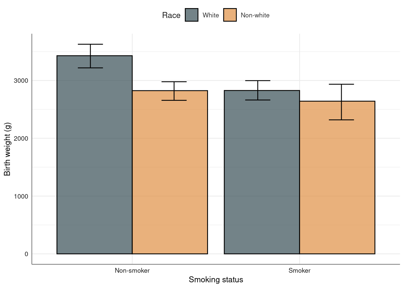
birthwt %>%
bar_error(bwt ~ smoke|Race) %>%
axis_labs()
No summary function supplied, defaulting to `mean_se()`
No summary function supplied, defaulting to `mean_se()`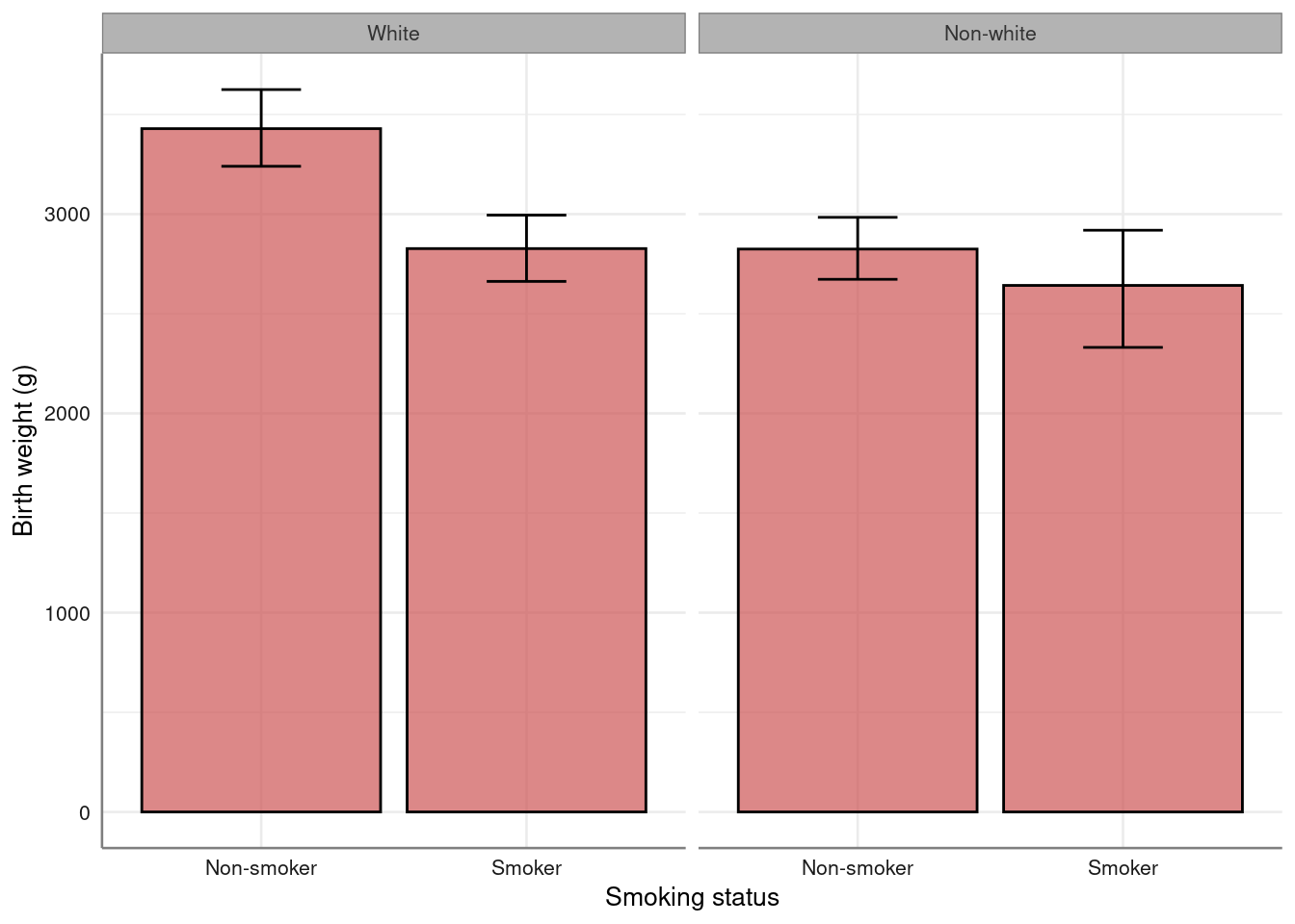 analysis of the linear model of smoking on birth weight, adjusting by race (and not by other potential confounders)
birthwt %>%
strip_error(bwt ~ smoke, pch = ~ Race, col = ~ Race) %>%
gf_refine(ggsci::scale_color_jama()) %>%
axis_labs()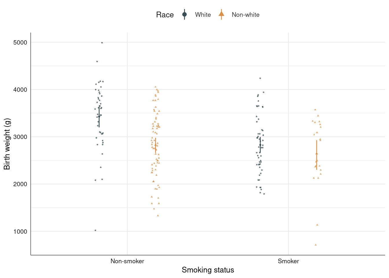 analysis of the linear model of smoking on birth weight, adjusting by race (and not by other potential confounders)
model_bwt <- lm(bwt ~ smoke + race, data = birthwt)

model_bwt %>%
glm_coef(labels = model_labels(model_bwt))| Parameter | Coefficient | Pr(>|t|) |
|---|---|---|
| Constant | 3334.95 (3036.11, 3633.78) | < 0.001 |
| Smoking status: Smoker | -428.73 (-667.02, -190.44) | < 0.001 |
| Race: Afican American | -450.36 (-750.31, -150.4) | 0.003 |
| Race: Other | -452.88 (-775.17, -130.58) | 0.006 |
Similar results can be obtained with the function tab_model from the sjPlot package.
sjPlot::tab_model(model_bwt, collapse.ci = TRUE)| Birth weight(g) | ||
|---|---|---|
| Predictors | Estimates | p |
| (Intercept) |
3334.95 (3153.89 – 3516.01) |
<0.001 |
| Smoking status: Smoker |
-428.73 (-643.86 – -213.60) |
<0.001 |
| Race: Afican American |
-450.36 (-752.45 – -148.27) |
0.004 |
| Race: Other |
-452.88 (-682.67 – -223.08) |
<0.001 |
| Observations | 189 | |
| R2 / R2 adjusted | 0.123 / 0.109 | |
pubh::multiple(model_bwt, ~ race)$df| contrast | estimate | SE | t.ratio | p.value | lower.CL | upper.CL |
|---|---|---|---|---|---|---|
| White - Afican American | 450.36 | 153.12 | 2.94 | 0.01 | 89.95 | 810.77 |
| White - Other | 452.88 | 116.48 | 3.89 | < 0.001 | 178.72 | 727.04 |
| Afican American - Other | 2.52 | 160.59 | 0.02 | 1 | -375.48 | 380.52 |
Some advantages of glm_coef over tab_model are:
- Script documents can be knitted to Word and LaTEX (+ (besides HTML).
- Uses robust standard errors by default. The option to not use robust standard errors is part of the arguments.
- Recognises some type of models that tab_model does not recognise.
Some advantages of tab_model over glm_coef are:
- Recognises labels from variables and use those labels to display the table.
- Includes some statistics about the model.
- It can display more than one model on the same output.
- Tables are more aesthetically appealing.
In the previous table of coefficients confidence intervals and p-values for race had not been adjusted for multiple comparisons. We use functions from the emmeans package to make the corrections.
multiple(model_bwt, ~ race)$fig_ci %>%
  gf_labs(x = "Difference in birth weights (g)")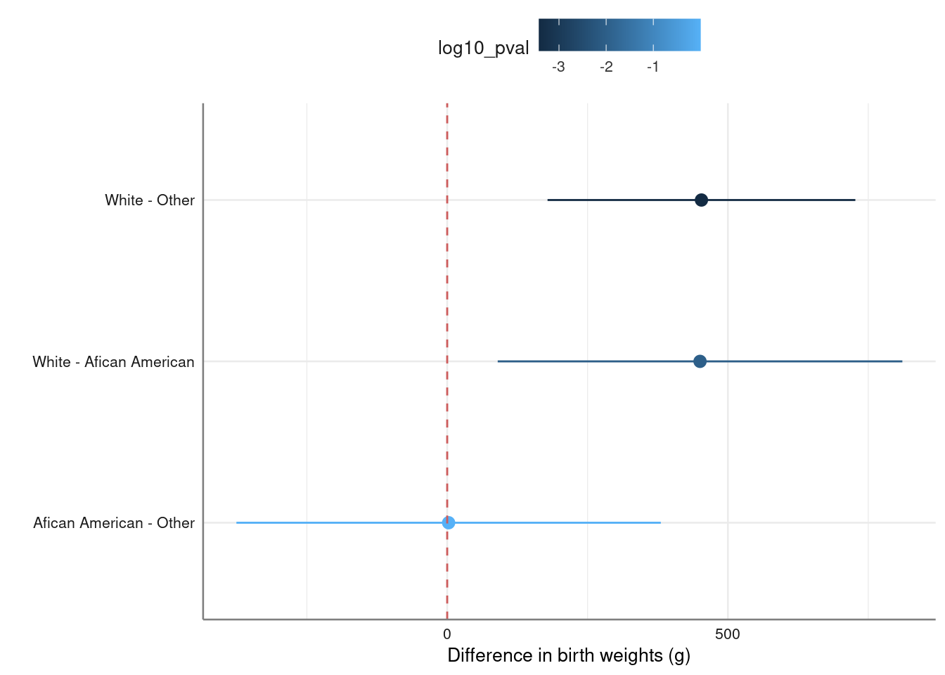
multiple(model_bwt, ~ race)$fig_pval %>%
  gf_labs(y = " ")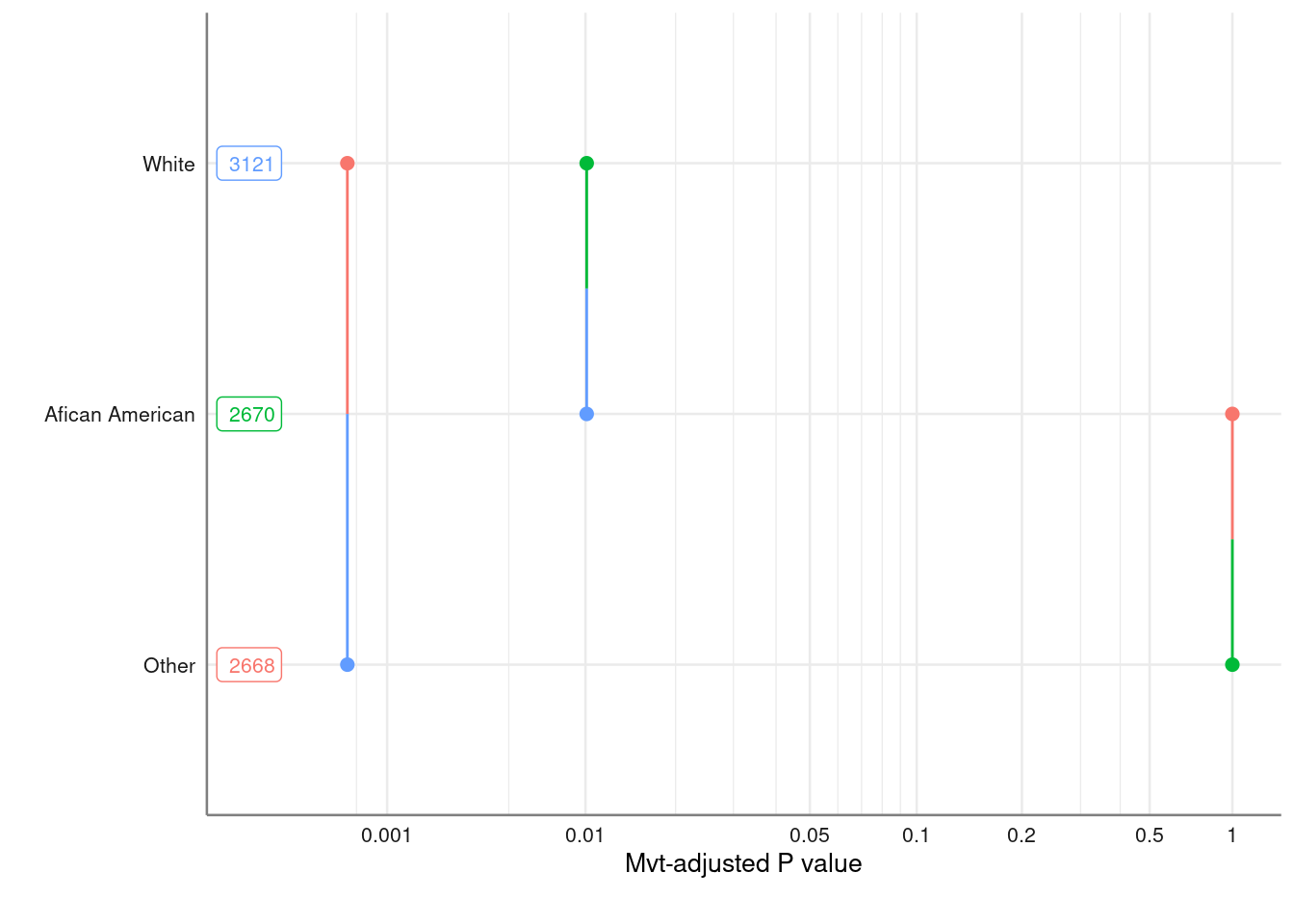
data(Bernard)
head(Bernard)| id | treat | race | fate | apache | o2del | followup | temp0 | temp10 |
|---|---|---|---|---|---|---|---|---|
| 1.00 | Placebo | White | Dead | 27.00 | 539.20 | 50.00 | 35.22 | 36.56 |
| 2.00 | Ibuprofen | African American | Alive | 14.00 | 720.00 | 38.67 | 37.56 | |
| 3.00 | Placebo | African American | Dead | 33.00 | 551.12 | 33.00 | 38.33 | |
| 4.00 | Ibuprofen | White | Alive | 3.00 | 1376.14 | 720.00 | 38.33 | 36.44 |
| 5.00 | Placebo | White | Alive | 5.00 | 720.00 | 38.56 | 37.56 | |
| 6.00 | Ibuprofen | White | Alive | 13.00 | 1523.39 | 720.00 | 38.17 | 38.17 |
Bernard %>%
  mutate(
    fate = relevel(fate, ref = "Dead"),
    treat = relevel(treat, ref = "Ibuprofen")
  ) %>%
  copy_labels(Bernard) %>%
pubh::cross_tab(fate ~ treat) | Mortality status | levels | Dead | Alive | Total |
|---|---|---|---|---|
| Total N (%) | 176 (38.7) | 279 (61.3) | 455 | |
| Treatment | Ibuprofen | 84 (47.7) | 140 (50.2) | 224 (49.2) |
| Placebo | 92 (52.3) | 139 (49.8) | 231 (50.8) |
dat <- matrix(c(84, 140 , 92, 139),
              nrow = 2, byrow = TRUE)
epiR::epi.2by2(as.table(dat))
             Outcome +    Outcome -      Total        Inc risk *        Odds
Exposed +           84          140        224              37.5       0.600
Exposed -           92          139        231              39.8       0.662
Total              176          279        455              38.7       0.631

Point estimates and 95% CIs:
-------------------------------------------------------------------
Inc risk ratio                               0.94 (0.75, 1.19)
Odds ratio                                   0.91 (0.62, 1.32)
Attrib risk *                                -2.33 (-11.27, 6.62)
Attrib risk in population *                  -1.15 (-8.88, 6.59)
Attrib fraction in exposed (%)               -6.20 (-33.90, 15.76)
Attrib fraction in population (%)            -2.96 (-15.01, 7.82)
-------------------------------------------------------------------
 Test that OR = 1: chi2(1) = 0.260 Pr>chi2 = 0.61
 Wald confidence limits
 CI: confidence interval
 * Outcomes per 100 population units
Bernard %>%
pubh::contingency(fate ~ treat)
Outcome
Predictor Dead Alive
Ibuprofen 84 140
Placebo 92 139
Outcome + Outcome - Total Inc risk * Odds
Exposed + 84 140 224 37.5 0.600
Exposed - 92 139 231 39.8 0.662
Total 176 279 455 38.7 0.631
Point estimates and 95% CIs:
-------------------------------------------------------------------
Inc risk ratio 0.94 (0.75, 1.19)
Odds ratio 0.91 (0.62, 1.32)
Attrib risk * -2.33 (-11.27, 6.62)
Attrib risk in population * -1.15 (-8.88, 6.59)
Attrib fraction in exposed (%) -6.20 (-33.90, 15.76)
Attrib fraction in population (%) -2.96 (-15.01, 7.82)
-------------------------------------------------------------------
Test that OR = 1: chi2(1) = 0.260 Pr>chi2 = 0.61
Wald confidence limits
CI: confidence interval
* Outcomes per 100 population units
Pearson's Chi-squared test with Yates' continuity correction
data: dat
X-squared = 0.17076, df = 1, p-value = 0.6794data(oswego, package = "epitools")
oswego <- oswego %>%
mutate(
ill = factor(ill, labels = c("No", "Yes")),
sex = factor(sex, labels = c("Female", "Male")),
chocolate.ice.cream = factor(chocolate.ice.cream, labels = c("No", "Yes"))
) %>%
var_labels(
ill = "Developed illness",
sex = "Sex",
chocolate.ice.cream = "Consumed chocolate ice cream"
)oswego %>%
mutate(
ill = relevel(ill, ref = "Yes"),
chocolate.ice.cream = relevel(chocolate.ice.cream, ref = "Yes")
) %>%
copy_labels(oswego) %>%
pubh::cross_tab(ill ~ sex + chocolate.ice.cream) | Developed illness | levels | Yes | No | Total |
|---|---|---|---|---|
| Total N (%) | 46 (61.3) | 29 (38.7) | 75 | |
| Sex | Female | 30 (65.2) | 14 (48.3) | 44 (58.7) |
| Male | 16 (34.8) | 15 (51.7) | 31 (41.3) | |
| Consumed chocolate ice cream | Yes | 25 (55.6) | 22 (75.9) | 47 (63.5) |
| No | 20 (44.4) | 7 (24.1) | 27 (36.5) |
oswego %>%
  pubh::mhor(ill ~ sex/chocolate.ice.cream)

                                   OR Lower.CI Upper.CI Pr(>|z|)
sexFemale:chocolate.ice.creamYes 0.47     0.11     2.06    0.318
sexMale:chocolate.ice.creamYes   0.24     0.05     1.13    0.072

                          Common OR Lower CI Upper CI Pr(>|z|)
Cochran-Mantel-Haenszel:       0.35     0.12     1.01    0.085

Test for effect modification (interaction): p =  0.5434
data(Oncho)
pubh::odds_trend(mf ~ agegrp, data = Oncho, angle = 0, hjust = 0.5)$fig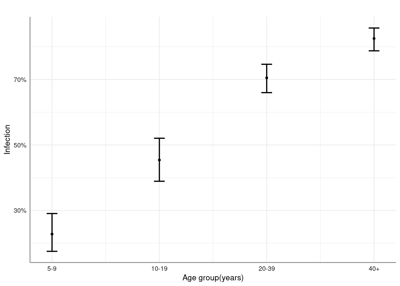 # Diagnostic test
Freq <- c(1739, 8, 51, 22)
BCG <- gl(2, 1, 4, labels=c("Negative", "Positive"))
Xray <- gl(2, 2, labels=c("Negative", "Positive"))
tb <- data.frame(Freq, BCG, Xray)
tb <- expand_df(tb)

pubh::diag_test(BCG ~ Xray, data = tb)
          Outcome +    Outcome -      Total
Test +           22           51         73
Test -            8         1739       1747
Total            30         1790       1820

Point estimates and 95 % CIs:
---------------------------------------------------------
Apparent prevalence                    0.04 (0.03, 0.05)
True prevalence                        0.02 (0.01, 0.02)
Sensitivity                            0.73 (0.54, 0.88)
Specificity                            0.97 (0.96, 0.98)
Positive predictive value              0.30 (0.20, 0.42)
Negative predictive value              1.00 (0.99, 1.00)
Positive likelihood ratio              25.74 (18.21, 36.38)
Negative likelihood ratio              0.27 (0.15, 0.50)
---------------------------------------------------------
pubh::diag_test2(22, 51, 8, 1739)
Outcome + Outcome - Total
Test + 22 51 73
Test - 8 1739 1747
Total 30 1790 1820
Point estimates and 95 % CIs:
---------------------------------------------------------
Apparent prevalence 0.04 (0.03, 0.05)
True prevalence 0.02 (0.01, 0.02)
Sensitivity 0.73 (0.54, 0.88)
Specificity 0.97 (0.96, 0.98)
Positive predictive value 0.30 (0.20, 0.42)
Negative predictive value 1.00 (0.99, 1.00)
Positive likelihood ratio 25.74 (18.21, 36.38)
Negative likelihood ratio 0.27 (0.15, 0.50)
---------------------------------------------------------